Once the Export Sales Format has been configured to export as a Pivot Table and an Export Sales Format File exists, the data can be displayed in Excel.
The steps outlined below will enable the Pivot Table Sales Format data to be displayed in an Excel Spreadsheet.
Note!
The steps outlined below will vary between different versions of Excel.
The purpose of this topic is to demonstrate the general process to add a PivotTable to an Excel Spreadsheet from an external data source.
Once the steps outlined below have been completed and a connection established with the Idealpos exported sales format, save the Excel Spreadsheet.
When the Excel Spreadsheet is opened, it will restore the connection to the data - the below process is only required for the initial setup.
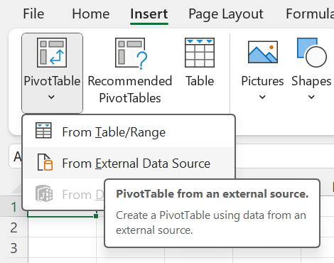
Create a new Excel Spreadsheet.
Within Excel, press the Insert tab > PivotTable (down arrow to show additional options) > From External Data Source.
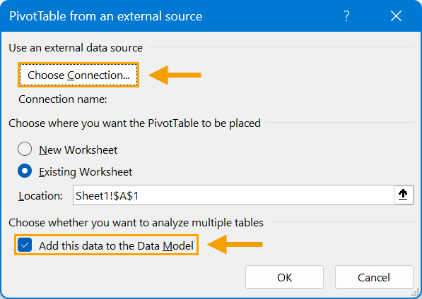
Enable "Add this data to the Data Model" > "Choose Connection"
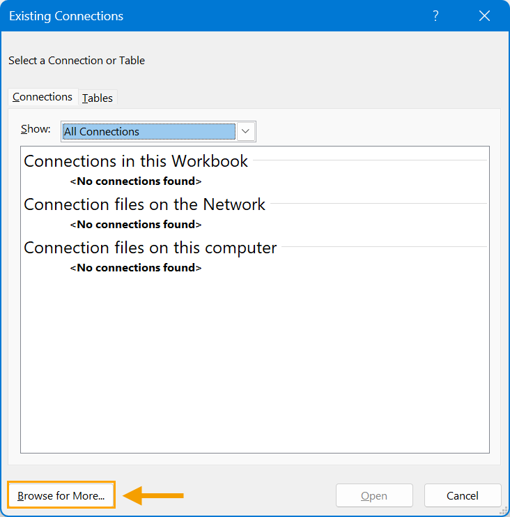
Browse for More
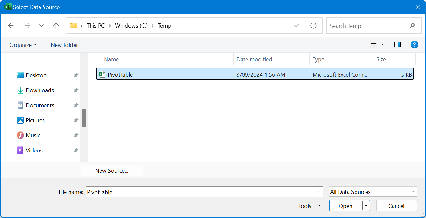
A Folder Browser window will open.
Browse to the Export Folder location configured in Idealpos earlier.
Once the file has been selected, press "Open".
The Text Import Wizard will appear.
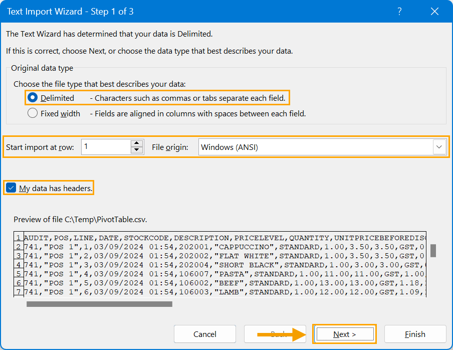
Step 1 of 3:
Ensure that the following options have been selected:
Original Data Type: Delimited
Start import at row: 1
File origin: Windows (ANSI)
My data has headers: Enable checkbox
Press "Next" to continue to the next step of the Text Import Wizard.
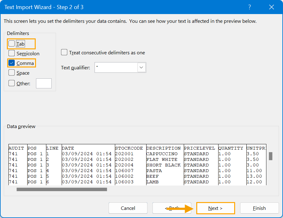
Step 2 of 3:
Untick the "Tab" Delimiter checkbox and enable the "Comma" checkbox.
Press "Next" to continue to the next step of the wizard.
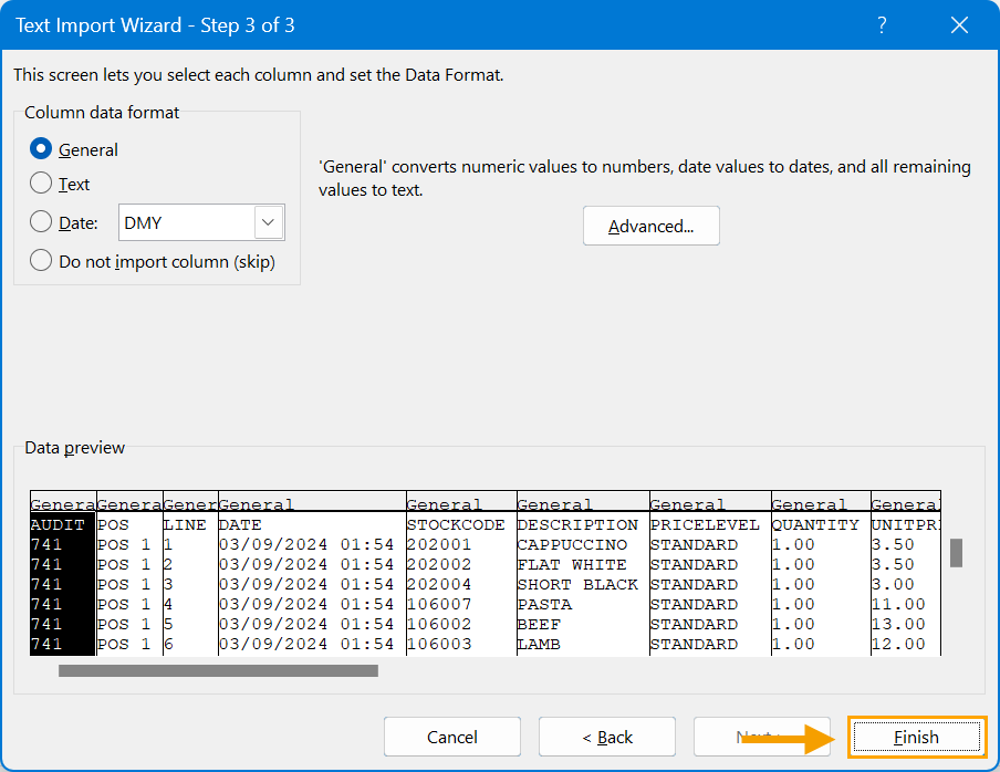
Step 3 of 3:
Leave the Column data format as General and press "Finish".
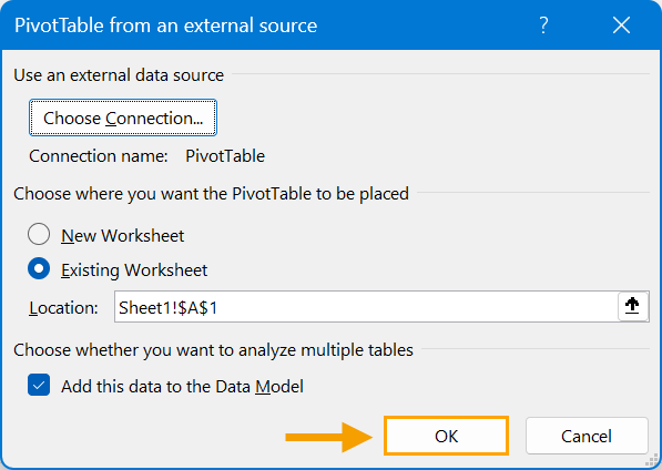
Press the "OK" button on the PivotTable from an external source window.
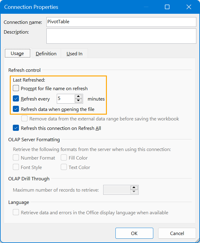
Even though the Data Source connection to the PivotTable data has now been created, a few more steps are required to configure the Refresh Control for the connection.
In Excel, press the "Data" tab and select "Queries & Connections".
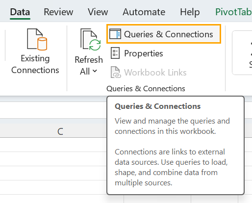
On the right-hand side of the Excel window, a "Queries & Connections" section will be displayed.
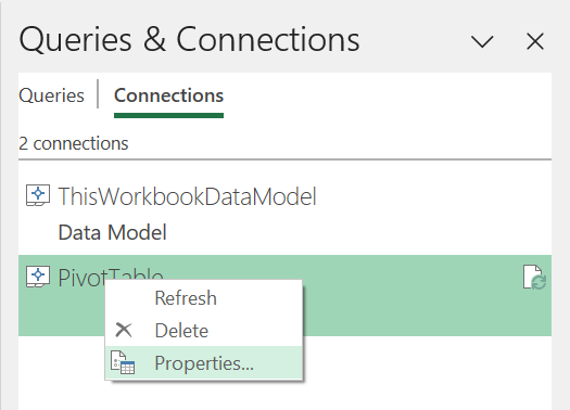
Ensure that "Connections" is selected, then right-click on the "PivotTable" and choose "Properties".
Set the options as follows > "OK":
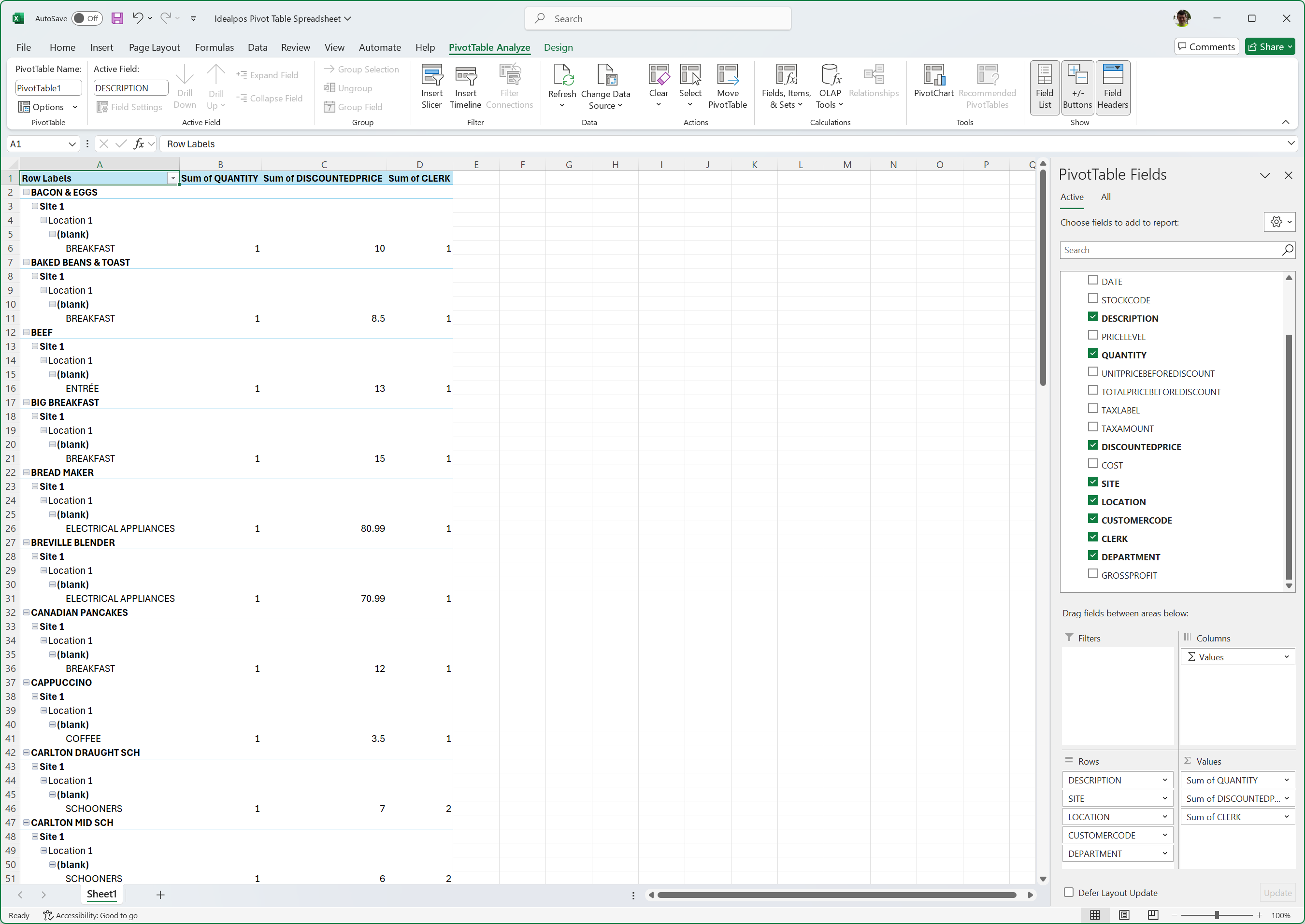
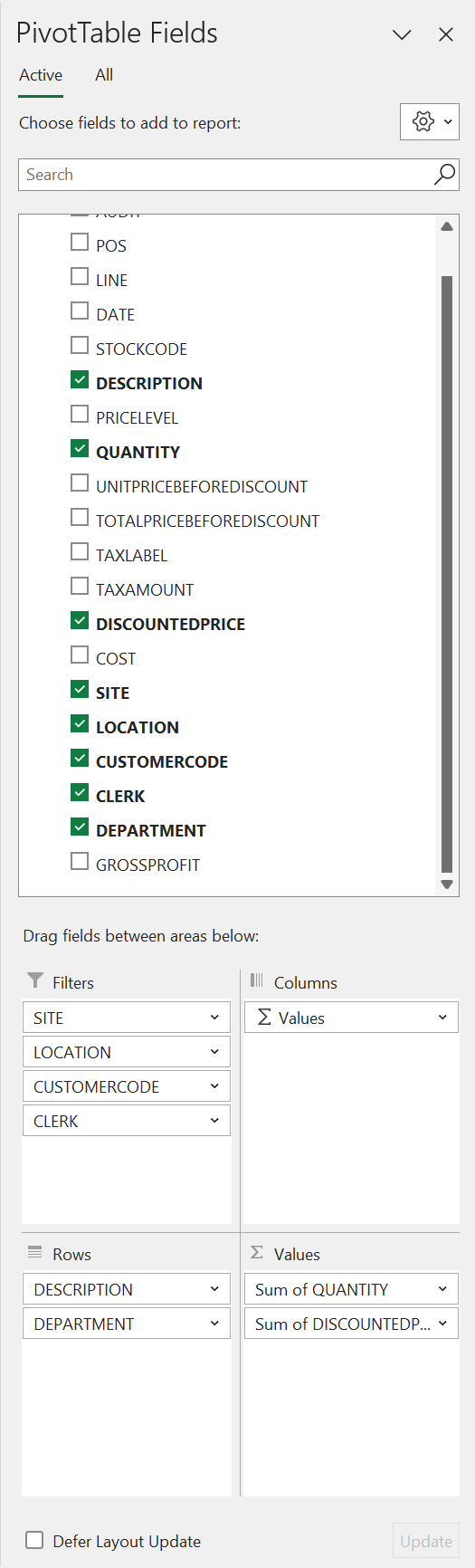
The fields for the PivotTable will need to be selected from the fields on the right-hand side of the Excel window.
Any fields that are required can be selected.
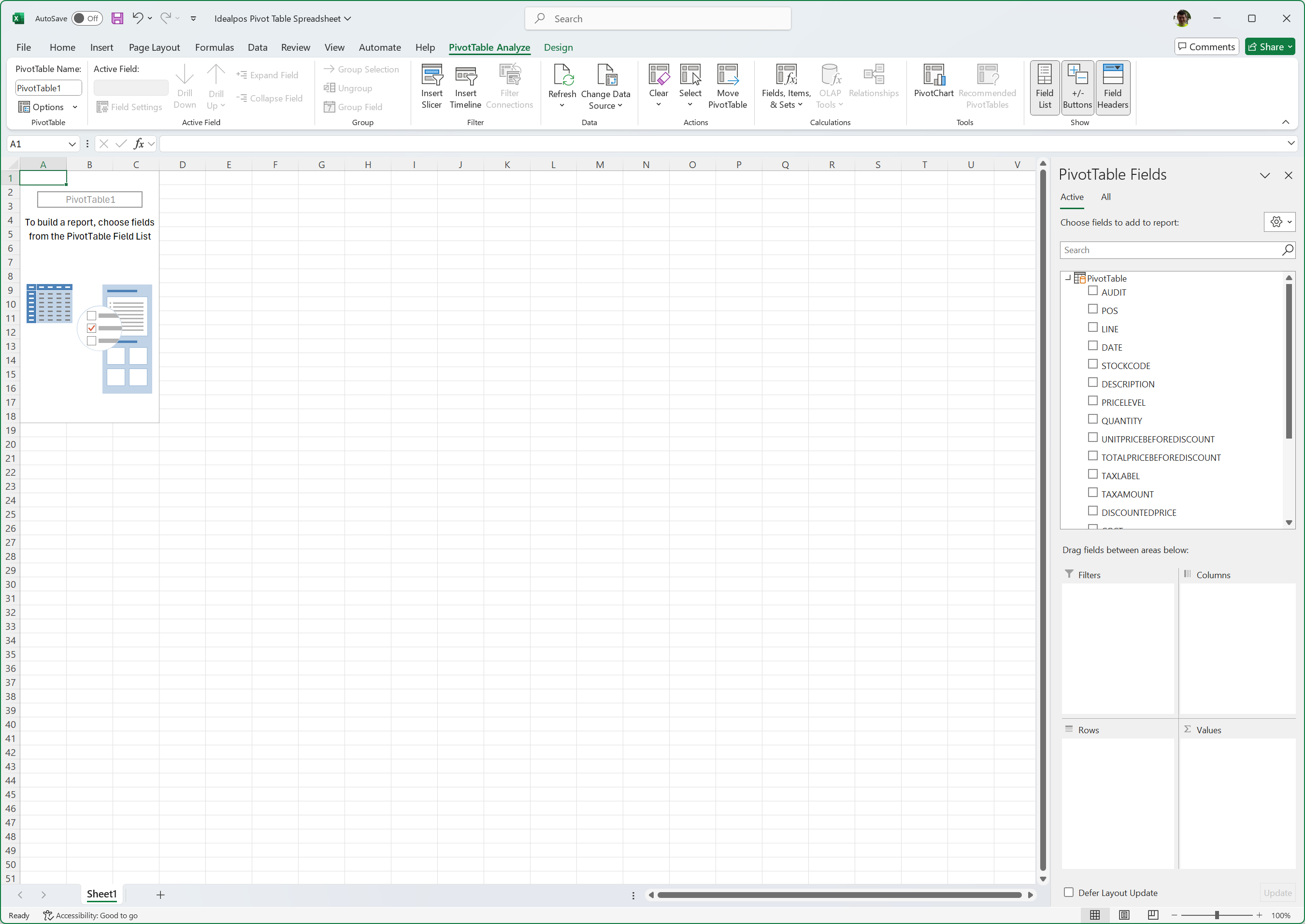
For the purposes of demonstrating this function, the below is an example set of fields that have been selected:
Description, Quantity, DiscountedPrice, Site, Location, CustomerCode, Clerk, Department.
After the required fields are checked/enabled, the Excel window will appear like the below example:
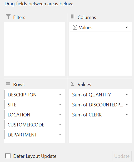
The below screenshot example shows suggested usage. This can vary depending on your requirements and any fields that are desired can be dragged to the Filters.
Before dragging the suggested fields to the Filters section | After dragging suggested fields to the Filters section:
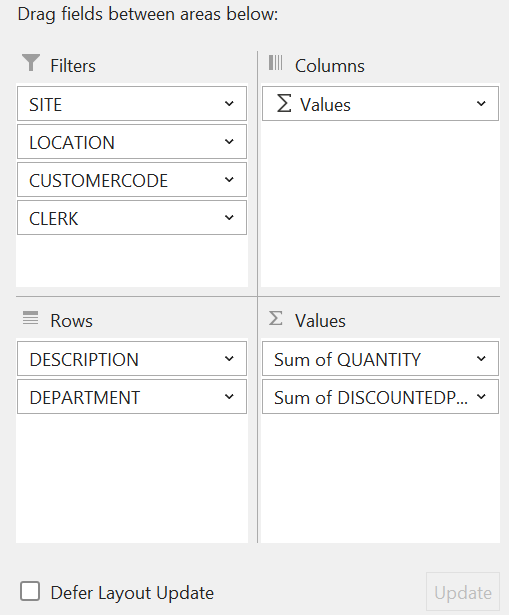
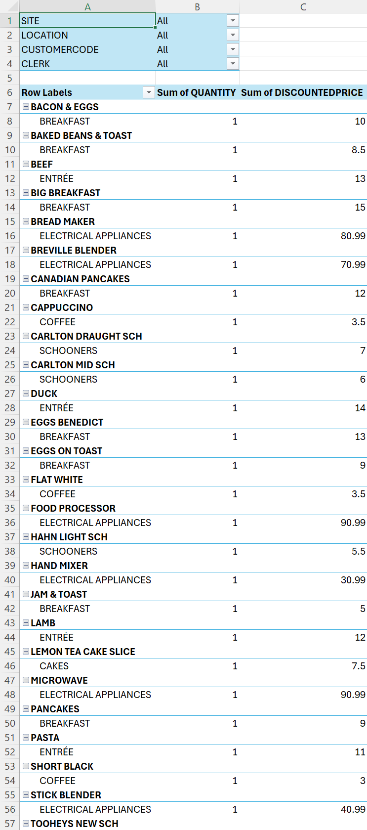
After the fields have been dragged into the Filters field, the Pivot Table will appear like the example below.
The table can be filtered as required via the dropdown boxes at the top of the table.
If the PivotTable Fields option is closed and further adjustments to the PivotTable Fields are required, the PivotTable Fields can be displayed again by clicking on the "PivotTable Analyze" tab in Excel, then selecting the Field List.
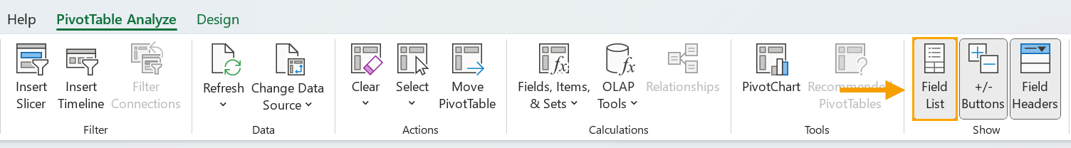
This will display the PivotTable Fields so they can be adjusted as required.
Once the above process has been completed and a connection is established, open the Excel Spreadsheet and the data will be refreshed as per the Refresh settings that were selected during the above process.